- Average
- Linear model
- Quadratic polynomial model
- Exponential model
- Which model is the best one?
- Multiple variable model
- Nonlinear models
- Creating charts
The application Online multiple regression calculator let you achieve a regression analysis on your sample of data.
Let's have a look at the data drawn in the below graph.
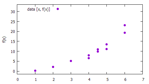
Sample data to be analysed. The data are generated but could be collected from an experiment. Note that the above plot is not a function as for one x more observed values f(x) can exist. The task is to find a mathematical function describing the dependency
If we would have only two points in the chart, then we would be able to find an exact line F(x) = a + bx passing each point. If we would have only three points in the chart, then we would be able to find an exact parabola F(x) = a + bx + cx2 passing each point. But we have over 10 points and finding a polynom of such order would be pointless.
1. Average
We can find the average which is depicted below. It is simple to determine average of all f(x). It doesn't seem to be much helpful though: the found solution doesn't fit the data well.
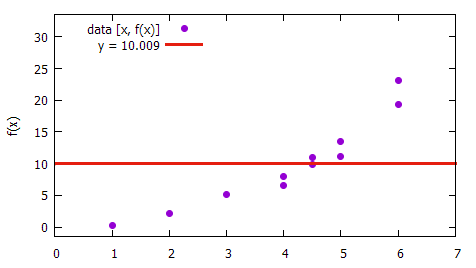
The average F(x) = 10.009 is easy to find but doesn't fit data well
2. Linear model
The data—with some degree of imperfection—are better represented by a line F(x) = a + bx. Both coefficients a and b has to be determined.
Popular calculators CASIO fx-991/fx-570 can find these coefficients: press [MODE] 3 (STAT), [AC] and then enter the sample data pairs [x, y]. Once finished, let's setup the regression analysis type to linear: [SHIFT] 1 STAT 1 (Type) 2 (a + bx). Then let you display the computed coefficient: [AC] [SHIFT] 1 STAT 7 (Reg) 1 (a) to get value a = -6.673. Similar way to get b = 4.078. So we got that F(x) = -6.673 + 4.078 x. You can alter the input data if you press [SHIFT] 1 2 (Data). To leave the regression mode: press [MODE] 1 (COMP).
And how does the description F(x) = -6.673 + 4.078 x looks like in the chart?

The linear description F(x) = -6.673 + 4.078 x fits the sample of data much better then the pure average
The CASIO calculator is useful but not that convenient and has its limits. The below online program is much more efficient. Either you enter the data into the fields (RHS is right hand side or simply f(x)) or you can directly paste the data into the textarea below the cells. The two ticks select functions which have to be involved in the analysis. In this case it is function F1(x) = 1 and F2(x) = x. The least square method finds that their combination expressed as F(x) = -6.674 + 4.078 * x fits the sample best.

The software brings us to the same solution we obtained from the calculator
3. Quadratic polynomial model
You likely expect to increase the degree of the function to the second degree polynomial so it becomes F(x) = a + bx + cx2. You still would have luck with the CASIO calculator but let's see how to use the program. By default, there is no x2 function available and that's why input line with button Insert exists. Let you insert either x*x or x2 and ensure that all three functions (1, x, x2) are ticked (to be included into the result). Supposed the data are entered, press button Solve.
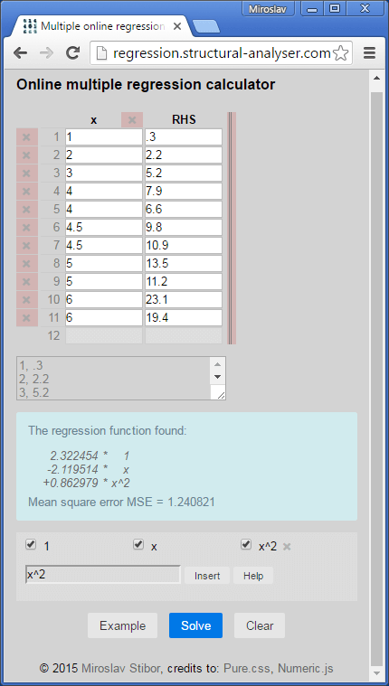
The coefficients are found such that the parabola F(x) = 2.322 - 2.12 x + 0.863 x2 fits the data best
4. Exponential model
Eventually as a part of this excercise let's substitute x2 guy by ex and make an illustrative plot then.
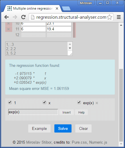
The program uses the method of least squares to find the function as F(x) = -1.975 + 2.09 x + 0.0265 ex
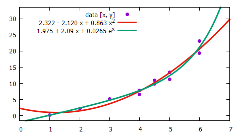
The sample data and their replacement by quadratic and exponential model
5. Which model is the best one?
There is no best model. The function F(x) has to consist of such terms, which describe the analysed model well. Since models usually some from the real world, there is known description but unknown coefficients. The coefficients can be determined by the method of least squares as the above used analyser does.
MSE (Mean square error)
The parameter MSE—which is being displayed as part of the results—tells us how close the approximation F(x) is from the data being studied. It is a parallel to standard deviation: the lower is the value, the better is usually description. So if we look aside the physical meaning, the exponential form fits the data better than the quadratic form (MSE = 1.06 vs 1.24).
6. Multiple variable model
You can enter and solve multiple dimensions as well:
Either enter the data directly into the textfield or use the red handler right from the cells to stretch the table, so more columns are available for your input.
7. Nonlinear models
The current implementation doesn't support nonlinear least square method. It means that
- you are able to find coefficients a1
and a2 if your model is
F(x) = a1 sin(x) + a2 ex. - But you won't be able to solve model if formed as
F(x) = sin(a1 x) + ea2 x.
8. Creating charts
The feature was considered but is not implemented in the current version. That might change in the future.
(c) 2016 Miroslav Stibor, back to the table of contents